Draw Tree 100 Thousand Leafs
Decision Tree for Better Usage
From Leaf, Tree, to Forest

When there are a ton of materials about Decision Tree, the reason for writing this posting is to give a chance to take a different look at the topic. Exposed to diverse ways of understanding is an effective learning method as if you touch something part by part and you know the whole shape. The topics you will see may fill what you are missing out on Decision Tree or you can simply brush up on what you already know. This posting starts with how Decision Tree works, covers basic characteristics, and extends it to the technique called Bagging.
Prerequisite
Some basic understanding of model evaluation, especially against testing set, will be more than helpful. You can refer to my previous posting which covers a part of it.
Contents
- How to split — How to measure impurity to base a split
- Continuous Features — How to find a split point on continuous values
- Non-linearity and Regression — Why it is non-linear and how to regress
- Greedy Algorithm — Why Decision Tree can't find the true optimum
- Tendency to Over-fit — Why over-fitting happens and how to prevent it
- Bagging and Random Forest — How Bagging works
- Demo in R — Loan Default data
How to Split
How Decision Tree works is basically about how to split nodes because this is how a tree is built. Let's assume that we have a binary classification problem; Cola vs. Soy Sauce. When you need to drink whichever you pick, you wouldn't make a decision just by looking. You would probably smell it or even taste a bit of it. So, color is not a useful feature but smell should be.
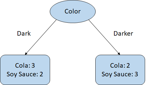
In the example, there are 5 cups for each, 10 in total, and your job is to classify them using your eyes. We say the left node decides on Cola because there are more Cola classes, and vise versa. The result wouldn't be promising, and you may end up drinking cups of soy sauce. In this case, the bottom nodes are not pure because the classes are almost equally mixed up.
When one class is dominant in a node, we say the node is "Pure".
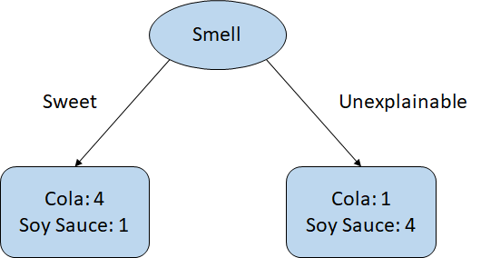
Now, you utilize your nose. You could still make some mistakes, but the result should be much better. Because the nodes mostly have a dominant class, Cola on the left and Soy Sauce on the right, this is purer. Then, the question becomes how to measure 'Purity'. The answer could be many, but we can talk about Gini.
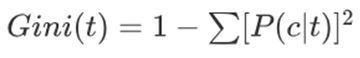
The formula is saying to add up all the squared probabilities of a class being correct on each node and deduct the sum from 1. Okay, let's take a look at some examples.
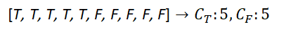
We have a node with 10 examples, 5 of them being True and 5 of them being False. Your decision on this node could be either True or False. Now, you know this node is not quite pure. To measure how not pure, we can calculate it as follows.

Out of 10, the probability of True class is 0.5 and the same for False class. In fact, this is the least pure case, proving that the highest Gini is 0.5. The following is another example.
Lower Gini is purer, so better.
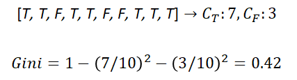
There are more True classes so you can claim your decision to be True more confidently. Likewise, Gini is now lower. Another question to make at this point is when to split. We know that 7 to 3 in the example is 0.42 in Gini, but we want to make it even purer and decide to split the 10 classes with another feature.
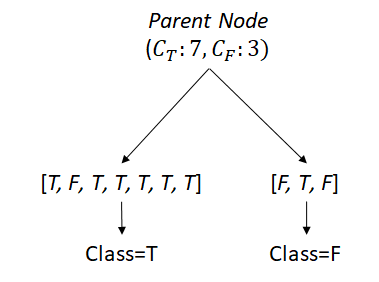
The split was made into 2 child nodes. Now, we say the left node is True with more True classes, and vise versa for the right node. We can measure the purity of each node, but how can we conclude one result to compare with the parent? We can simply give them weights by node size to parent total.
We say a split gains "Information" if Gini decreases.

The Gini 0.3 is smaller than 0.42 of the parent, thus, the split gained some information. It would be great if some split results the following.
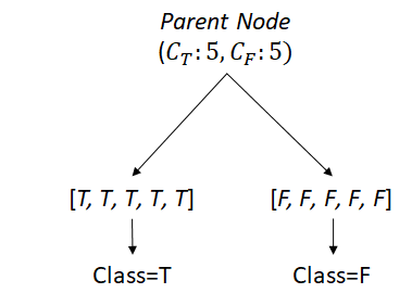
Parent is so bad its Gini is 0.5, but one split can decrease it to 0. Notice the two children are doing perfect jobs to classify True or False. It seems like splitting is always helpful, however, that is not true.
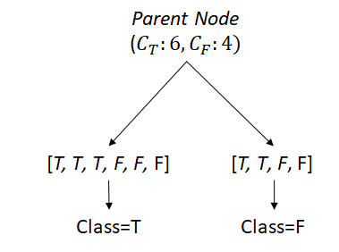
We know intuitively the parent node's Gini is not the maximum (0.5), but the children's are. In other words, the split made it worse (lost information). Even if the Gini's are the same for a parent and its children, this is still worse because the model with more nodes means more complications. Indeed, modern Decision Tree models damage it by adding more nodes.
One more thing to note is that Gini is not the only one to measure purity. There are many others, but the following two are worth mentioning.
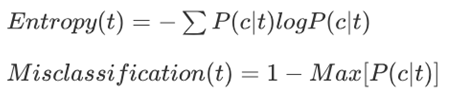
You can try those as we did for Gini, and it will output different results. Then, which one is better than the others? The answer is 'it depends'. We should rather focus on how they are different.
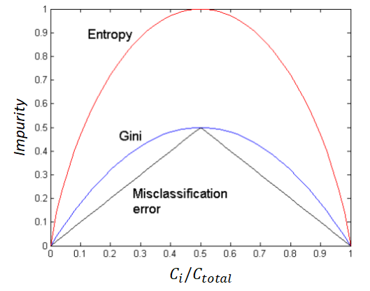
We learnt that the maximum of Gini is 0.5 which is different than that of Entropy. Namely, Entropy hikes up more sharply than Gini. This means it can penalize an impure node harder.
Another difference is that Misclassification Error is not smooth like the other two. For example, an increase on the x-axis from 0.1 to 0.2 adds the same impurity as an increase from 0.3 to 0.4, which is linear. On the contrary, Gini sees impurity at 0.4 as almost same as impurity at 0.5, so does even more Entropy. This means Gini and Entropy are stricter against impurity. And which one to use depends on the situation.
Continuous Features
We started with categorical features, and this probably didn't strike anyone as strange. But Decision Tree can handle continuous features gracefully. Let's take a look at the example.
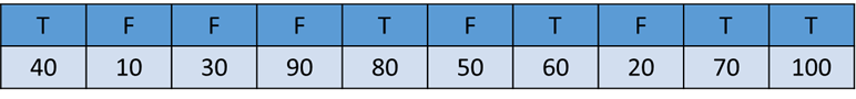
We have a series of values; 10, 20, …, 100, each of which is labeled as True or False. First thing to do is ordering them, and we can grab a point between some two values. Let's say we split at 45.
Theoretically, there are infinite choices to split continuous values.
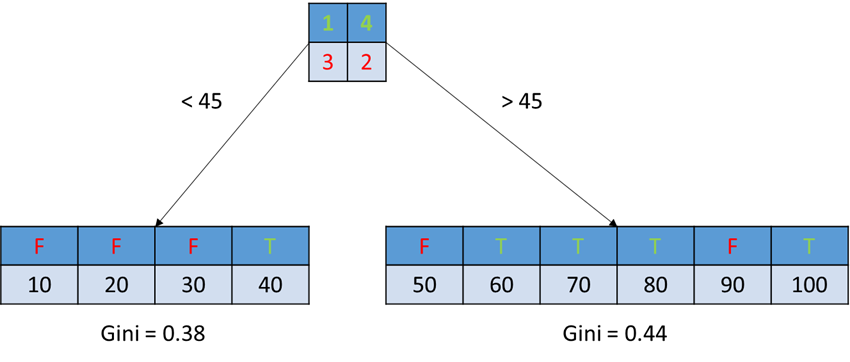
There are four values less than 45, and three of them are False with one of them True. The same rule is applied to the right greater than 45. Now, we can calculate the Gini for each group. Of course, we need to put weights on them to get the final Gini. We do this to all split points possible between values.
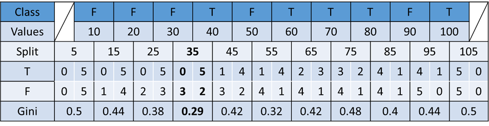
As seen on the table, the lowest Gini is at the split point 35 of which the left is perfectly pure (all False classes) and the right has 7 classes with 5 of them being True classes. The calculation seems to be tiring, but when you slide through the values the True or False counts change one by one. This means that each calculation only needs to make a slight change for the next calculation (machines do that for us, anyway). In conclusion, continuous features are handled very similarly with categorical features but with more calculation.
Non-linearity and Regression
Straight to the point, Decision Tree is a non-linear model. If an example is classified by a feature node, how much doesn't matter.
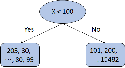
In the figure, there are some extreme values like -205 or 15482. However, they all belong to just one node with any other number satisfying the condition. They don't get any special titles such as 'Super Yes' or 'Double No'. At this point, Decision Tree seems to be unable to do regression. But yes, it can.
Let's look at some analogies. We all know that an ANOVA model can do regression in which averages of categorical predictors represent certain group of samples. A similar idea can be applied to Decision Tree.
Some statistics such as mean or median of examples in a node can represent the node
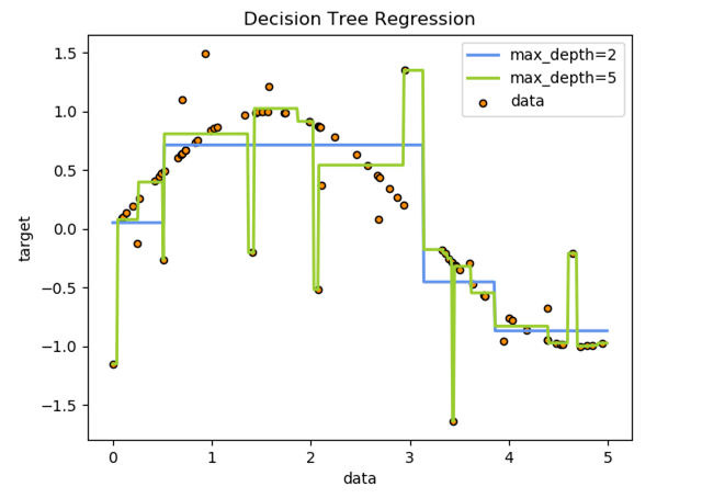
First, it is obvious that Decision Tree is non-linear from the box-like lines. One more takeaway here is that it shows how Decision Tree can over-fit examples. 'Max-depth' controls how complex a tree can be built. We can see that a tree with Max-depth set to 5 is trying so hard to fit all the far-off examples at the cost of the model being so complex.
Greedy Algorithm
Decision Tree is a greedy algorithm which finds the best solution at each step. In other words, it may not find the global best solution. When there are multiple features, Decision Tree loops through the features to start with the best one that splits the target classes in the purest manner (lowest Gini or most information gain). And it keeps doing it until there is no more feature or splitting is meaningless. Why does this sometimes fail to find the true best solution?
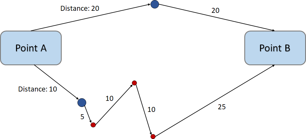
To understand what is actually happening to 'Greedy' manner, we assume that we are going from Point A to Point B. On a greedy standard, we don't see the red way-points on Point A but only see the blue points. Standing on Point A, we decide the bottom because this is shorter than the top. But in the next step, we find the red point, and so on, ending up with a longer trip.
The best choice made at each step does not guarantee the global best.
The same could happen in Decision Tree because it doesn't combine all the possible pairs. Imagine there are hundreds of features if not thousands, categorical and continuous mixed, each of which has all different values and ranges. Mixing them up all the way possible should be prohibitive. Knowing that Decision Tree is greedy is important to understand why the advanced methods like Bagging works.
Tendency to Over-fit
Like every other model, Decision Tree has an issue with over-fitting. It could be a bit worse than other models in a way. An extreme example is an ID feature. We never want to use this as a feature anyway, but let's consider it as such for understanding.
It will keep trying to split if there remains any features to do so
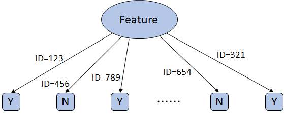
This is a multi-way split where each ID has a branch and each node has only one case to make decision since ID's are unique. Now, it becomes a look-up table. This is merely a bunch of hard-coded 'if statement'. The problem arises when it sees a new example. Then, the model will blow up because it doesn't have any function in it. If it was a binary split Decision Tree, it would be so deep as the number of examples.
Realistically, we won't ever use an ID as a feature, but this kind of event could still happen if a feature has a variety of values that can draw so many subtle boundaries or we let it grow in depth as much as it needs to fit all examples. There are also multiple ways to prevent this. Pruning is one of them which keeps a tree from growing deeper.
"Pre-pruning" controls the number of examples each node must have to split further. "Post-pruning" lets it expand, then finds over-fitting nodes.
In a more sophisticated way, we can consider Ensemble methods which let multiple learners make individual decisions and put them together for the final decision.
Bagging and Random Forest
Bootstrap aggregating, so called Bagging, an Ensemble model in which there are multiple learners. Its goal is to prevent over-fitting and find a better solution. As we can guess from its name, it utilizes the Bootstrap sampling method, which means that we draw samples 'with replacement'.
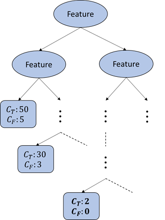
This is another example of over-fitting where the bottom node is split too much only to fit 2 examples. So, the two examples must be very exceptional in that all the upper nodes failed to uniquely separate them. Again, the node is now like a look-up table. What if we don't include the 2 examples when building a tree?
Bagging draws samples at random, letting some drawn more or some not drawn at all
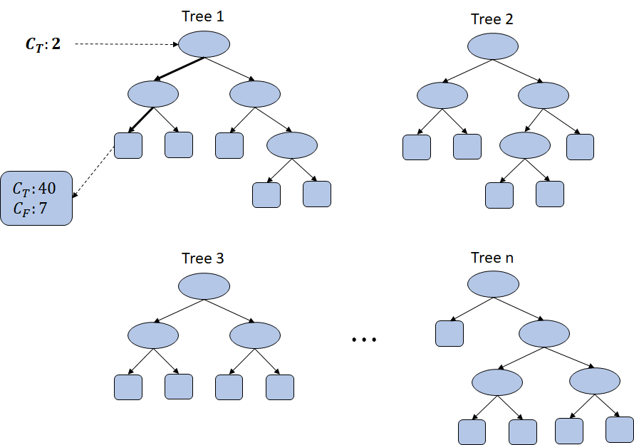
Tree 1 is built without the two exceptional examples. Now, we give it the two exceptions for testing, and it lands on a node with many examples. This no longer works like a look-up table simply because it didn't even see the examples. They could still be exceptional in other trees, but the final decision is made by all the 'n' trees voting. In short, random sampling prevents a model from memorizing examples and focuses on a general consensus.
Bagging can select features at random as well.
What if we apply Bagging to features? What it means is randomly selecting some features, not all. For example, we have 100 features and should guess some classes. We can use all of them as pure Decision Tree does, but we choose just some of them at random like using only 30 or 50 or any. It sounds so strange because it looks like we are not making full use of features.
Remembering the Greedy algorithm example of finding a shorter route, what if we didn't even have the choice of the bottom route? Because we didn't know that route, we would have gone with the top route that would result in a shorter trip overall.
By having less features, we can prevent a combination of features which leads to a local optimum but not the global.
By the nature of random selection, some feature set may result in the worse. That is why we should repeat so many times the random sampling as well as random feature selection so it can find the best of combination biased toward general decision standards. But this may still not be the true global best because randomizing all these doesn't mean we go through all the possibilities yet (NP-Complete problem).
One thing to note is that Bagging is an Ensemble method that can be applied to any model, not just Decision Tree. When Bagging is applied to Decision Tree, it becomes Random Forest just like trees comprise a forest.
Demo in R
Loan dataset is intuitive and easy to understand. We have 300 examples and 11 features such as Age, Gender, Loan Amount, Income, and Loan Status as the target. This is a binary classification guessing a loan to be in default or not.
The code uses the minimum libraries so it can focus on simulations. Also, Cross-validation was not used for evaluation to keep it simple (still fair because the same training/testing set were used for all the models). The full code and the data can be found on Github.
- Full Model — Evaluated against Training Set
          # Classification model with all features
clf <- rpart(formula = Loan_Status ~., data = training.set,
            control = rpart.control(minsplit = 1))          # Predict from training set and calculate accuracy
pred <- predict(clf, newdata = training.set[, -12], type = 'class')
round(sum(training.set[, 12]==pred)/length(pred), 2)          # Plot the tree
rpart.plot(clf, box.palette = 'RdBu', nn = T)
The model was built using all of the features, and it was tested against the training set, not the testing set. This was intended to see how over-fitting would happen.
*Words on the graph may not be legible but not important at this point. Please focus on the shape especially the depth and the number of nodes.
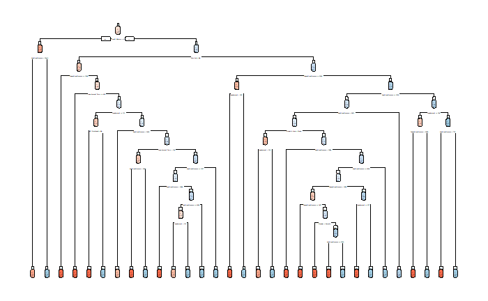
The tree is so deep and complex. Its accuracy is 0.96, almost perfect, but tested against its own training set. Now, let's evaluate the model against the testing set (unseen data).
- Full Model — Evaluated against Testing Set
          # Evaluate against testing set
pred <- predict(clf,            newdata = testing.set[-12], type = 'class')
round(sum(testing.set[, 12]==pred)/length(pred), 2)
Note that the parameter 'newdata' is now 'testing.set'. The result is 0.63 which is much less than what's tested against the training set. This means that the model using all features and all examples didn't successfully generalize it.
One thing we can do here first is to tweak the parameter. Limiting the depth can be helpful because the model won't grow that deep, preventing over-fitting. All accuracy hereafter is calculated from the testing set.
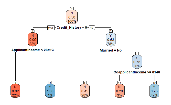
- Full Model with Depth Limit
          # Set maxdepth to 3
clf <- rpart(formula = Loan_Status ~., data = training.set,
            control = rpart.control(minsplit = 1,            maxdepth = 3))          # Evaluate against testing set
pred <- predict(clf, newdata = testing.set[-12], type = 'class')
round(sum(testing.set[, 12]==pred)/length(pred), 2)
Evaluated against the testing set, the accuracy is now 0.68 which is higher than 0.63. Also, the tree is a lot simpler without even using all of the features.
- Reduced Model with Random Sampling — Random Forest
          # Build 100 trees with max node
clf <- randomForest(x = training.set[-12],
            y = training.set$Loan_Status,
            ntree = 100,            maxnodes = 5)
We build 100 trees with up to 5 maximum nodes for each. The accuracy is 0.72, higher than ever. This means that the model found some way to handle exceptional examples. When we want to improve it even more, should we just increase the number of trees? Unfortunately, it might not be too helpful as Random Forest is not magic. If lucky enough, it could be amazingly better only until it sees completely new data.
The improvement is based on a consensus, meaning that it gives up on minor examples in order to fit more general examples.
Conclusion
We learnt the fundamentals of Decision Tree, focusing on the split. This was shown for both categorical and continuous values. Also, we checked out some characteristics of Decision Tree such as non-linearity, ability of regression, and greedy algorithm. For over-fitting, controlling depth and Bagging were introduced with the demo in R.
In the real world, these wouldn't always be working because we shouldn't expect data to come as clean as we wish they were. However, knowing these properties and parameters will be a good start for creative tries.
Good Reads
- Introduction to Data Mining: Chapter 4. Classification
- Scikit-Learn Example: Decision Tree Regression
- Random Forest Video Guide: Introduction to basic ideas
- 'rpart' R Library: Tutorial and more details
- 'randomForest R Library: Simple tutorial
You are encouraged to put forward your opinion. Comment here! Or talk to me via LinkedIn if you'd like to point out something wrong on this posting quietly… Also, you're welcome to visit my portfolio website!
Source: https://towardsdatascience.com/decision-tree-for-better-usage-622c025ffeeb
0 Response to "Draw Tree 100 Thousand Leafs"
Post a Comment